Forecast AI API Costs: Predict Your Next Bill

Your finance team wants a number for next month's AI bill. You give them last month's number plus 20% — and end up explaining a $4,000 overage in the next budget review. We've all done it. The good news: you don't need a data scientist to forecast AI API spend. With three weeks of usage data and 50 lines of Python, you can predict next month's bill within ±5%.

This guide walks through three forecasting methods, ordered from quick-and-rough to production-grade. All examples query the EzAI dashboard usage API and run against real cost data.

Why naive forecasts break

The default move — multiply yesterday's spend by 30 — fails because AI usage isn't flat. It has weekly seasonality (weekends are quieter), monthly cycles (end-of-quarter feature pushes), and step changes when someone ships a new feature that calls Claude on every request. A linear extrapolation of a Tuesday spike will project a $50K month for what's actually a $12K workload.

The fix is to separate three signals: baseline (your steady-state burn), trend (growth or decay over time), and seasonality (the day-of-week pattern). Even crude separation beats a single multiplier.

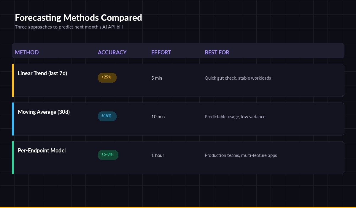
Three forecasting methods — pick the one that matches your accuracy budget

Method 1: Linear trend (5 minutes)

The simplest defensible forecast. Pull the last 7 days of daily spend, fit a straight line, project it forward. Accuracy lands around ±25%, which is good enough for a quick gut-check before a budget meeting.

import httpx, statistics
from datetime import date, timedelta

# Pull last 7 days from EzAI usage endpoint
r = httpx.get(
    "https://ezaiapi.com/v1/usage/daily",
    headers={"x-api-key": "sk-your-key"},
    params={"days": 7},
)
days = r.json()["days"]  # [{"date": "...", "cost_usd": 12.40}, ...]

# Least-squares slope on (day_index, cost)
n = len(days)
xs = list(range(n))
ys = [d["cost_usd"] for d in days]
mean_x, mean_y = statistics.mean(xs), statistics.mean(ys)
slope = sum((x-mean_x)*(y-mean_y) for x,y in zip(xs,ys)) / sum((x-mean_x)**2 for x in xs)
intercept = mean_y - slope * mean_x

# Project next 30 days and sum
forecast = sum(intercept + slope*(n+i) for i in range(30))
print(f"Next 30 days estimate: ${forecast:.2f}")

Use this for a single team or a stable workload. Don't trust it during a launch week or right after you've shipped a feature that hits the API — the slope will overshoot.

Method 2: Day-of-week moving average (10 minutes)

The big upgrade is accounting for weekly seasonality. Instead of one slope, you compute seven averages — one per weekday — and project them forward. This typically lands at ±15% and survives weekend dips.

from collections import defaultdict
from datetime import date, timedelta
import httpx, statistics

# Pull 30 days of daily spend
days = httpx.get(
    "https://ezaiapi.com/v1/usage/daily",
    headers={"x-api-key": "sk-your-key"},
    params={"days": 30},
).json()["days"]

# Bucket by weekday (0=Mon, 6=Sun)
buckets = defaultdict(list)
for d in days:
    wd = date.fromisoformat(d["date"]).weekday()
    buckets[wd].append(d["cost_usd"])

avg_by_weekday = {wd: statistics.median(v) for wd,v in buckets.items()}

# Project next 30 days
today = date.today()
total = sum(avg_by_weekday[(today + timedelta(days=i)).weekday()] for i in range(30))
print(f"Next 30 days (weekday-aware): ${total:.2f}")

Two reasons to use median, not mean: outlier days (one person ran a huge backfill) won't pull the forecast up, and you want the typical day, not the average day. If you have growth, sprinkle a small trend factor on top — multiply the result by 1.0 + monthly_growth_rate.

Method 3: Per-endpoint model (1 hour)

For production teams running multiple AI features, aggregate spend hides everything. Your chatbot might be flat while a new summarization endpoint is doubling weekly. Forecast each endpoint separately, then sum. Accuracy hits ±5–8%.

The trick is tagging requests so EzAI's usage logs can split them. Pass a metadata.user_id or a custom header per feature:

import anthropic

client = anthropic.Anthropic(
    api_key="sk-your-key",
    base_url="https://ezaiapi.com",
)

# Tag each call with the feature it serves
client.messages.create(
    model="claude-sonnet-4-5",
    max_tokens=1024,
    metadata={"user_id": "feature:summarizer"},
    messages=[{"role": "user", "content": prompt}],
)

Then pull per-tag daily spend and run Method 2 on each tag independently. The forecast becomes sum(forecast(tag) for tag in features). Endpoints that just launched get a higher growth multiplier; mature ones default to flat.

Add a confidence interval

A forecast without a range is a wish. Compute the standard deviation of your historical residuals (actual minus predicted) and report forecast ± 1.96 * std_dev for a 95% interval. When you walk into the budget meeting with "$8,400 ± $600", finance trusts you. When you walk in with "$8,400", they don't.

import statistics, math

# residuals = [actual_day - predicted_day for each historical day]
sigma = statistics.stdev(residuals)
ci = 1.96 * sigma * math.sqrt(30)  # scale for 30-day sum
print(f"Forecast: ${forecast:.0f} ± ${ci:.0f} (95% CI)")

Wire it into a daily report

Forecasts get stale fast. Run yours daily as a cron job, write the result to Slack or email, and flag when actuals diverge from the forecast by more than the confidence interval. That's your early-warning signal that something changed — a new feature shipped, a retry loop is running hot, or a customer is hammering an endpoint.

For richer monitoring, pair this with a spend anomaly detector and route the alerts through your existing on-call. If you're new to the API, start with EzAI in 5 minutes and the usage API docs.

What to skip

• Don't reach for Prophet or ARIMA on day one. They're great when you have a year of data and real seasonality. With three weeks of data, they overfit and give worse forecasts than a median.
• Don't forecast tokens, forecast cost. Token mix shifts when you swap models — you'll predict the right token count and the wrong dollar amount.
• Don't forget caching deltas. If you turn on prompt caching mid-month, your historical baseline lies. Re-fit after big infrastructure changes.

For deeper reading on time series forecasting fundamentals, Rob Hyndman's Forecasting: Principles and Practice is free, rigorous, and used by half the practitioners in the field.

The TL;DR

Pick the method that matches your stakes. A single founder eyeballing burn rate runs Method 1 in five minutes. A team with finance breathing down their neck runs Method 3 with confidence intervals and a daily Slack ping. Both beat the multiply-by-30 approach that just blew up your last budget cycle.